Logistic regression
(This post is also available as a Jupyter notebook file here)
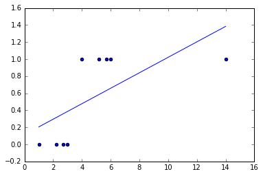
There are cases when linear regression simply doesn’t cut it. Classification tasks are classical examples for which a linear regression approach wouldn’t suffice.
Consider the following case as a classification task where we’re interested in the probability
\[h_\theta(x) = P(y=1| x ; \theta)\]If \(h_\theta(x) \ge 0.5\) we consider the sample as verifying the hypothesis.
%matplotlib inline
import matplotlib.pyplot as plt
import numpy as np

def genClassificationData():
    x = np.zeros(shape=9)
    y = np.zeros(shape=9)

    # Empirically adjusted for clarity's sake
    x[0] = 1
    x[1] = 2.2
    x[2] = 2.7
    x[3] = 3
    y[0] = y[1] = y[2] = y[3] = 0

    x[4] = 4
    x[5] = 5.2
    x[6] = 5.7
    x[7] = 6
    y[4] = y[5] = y[6] = y[7] = 1

    x[8] = 14
    y[8] = 1

    return x, y

def normEquation(x, y):
    ll = []
    for sample in x:
        ll += [[1] + [sample]]
    X = np.matrix(ll)
    ll = [[sample] for sample in y]
    y = np.matrix(ll)
    x_trans = X.T
    A = (x_trans * X).I
    theta = A * x_trans * y
    return theta

def plotLinearPredictor(x, y, theta):
    plt.figure()
    plt.scatter(x, y)

    y_regression = np.zeros(len(x))
    for sample in range(0, len(x)):
        y_regression[sample] = theta[0] + theta[1] * x[sample]

    plt.plot(x, y_regression)
    plt.show()

x, y = genClassificationData()
theta_coefficients = normEquation(x, y)
plotLinearPredictor(x,y, theta_coefficients)
Establishing decision boundaries
Ideally for a well-trained binary classifier we would like to be able to tell if a sample \(P\) lies in the region that verifies our hypothesis. For a parametric one-degree polynomial this is trivially \(\theta_0 + \theta_1 x_1 + \theta_2 x_2 \ge 0\).
Let us define \(h_{\theta}(x) = g(\theta^{T}x)\) and consider
\[g(x) = \frac{1}{1+e^{-x}}\]this is known as the sigmoid or logistic function.
sigmoid = lambda x: 1.0 / (1.0 + np.exp(-x))
plt.figure()
x = [float(i)/10 for i in range(-100, 100)]
y = [sigmoid(i) for i in x]
plt.plot(x, y)
plt.show()
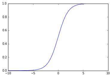
We can now interpret the hypothesis’ output as a function of the sigmoid parametrized by \(\theta\).
Convexity of the cost function
Applying gradient descent or another method that relies on the convexity of the search function will not work with logistic regression if we’re to use the same cost function
\[J(h_\theta(x), y)=\sum^{m}_{i=1}{(h_\theta(x^{(i)}) - y^{(i)})^2}\]since we’re now using a nonlinear function. We need to encode two considerations into a mathematical expression:
-
\[\begin{aligned} P(y=1|x;\theta) = 0 \wedge y = 1 \end{aligned}\]
In this case penalty process has to take place (large cost)
-
\[\begin{aligned} P(y=1|x;\theta) = 1 \wedge y = 0 \end{aligned}\]
Conversely, a similar penalty is needed
Therefore
\[J(h_\theta(x), y)=-\frac{1}{m}\sum^{m}_{i=1}{y^{(i)}log(h_\theta(x^{(i)})) + (1 - y^{(i)})log(1 - h_\theta(x^{(i)}))}\]This formulation has the following additional advantage
\[\frac{\partial}{\partial \theta_j}J(h_\theta(x), y) = \frac{1}{m} \sum^{m}_{i=1}{(h_\theta(x^{(i)}) - y^{(i)}) x_j^{(i)}}\]this grants us the same formulation as the linear case.
Multiclass classification
Classification can occur among many different classes. Two approaches are commonly used:
- one vs. all
- one vs. many
In the first approach the problem is decomposed into a number of binary classification problems that can in turn be solved via logistic regression. Given \(k\) classes a problem needs to be solved via binary classification \(k\) times. In the latter approach a classifier is constructed for each binary subset (generally slower).
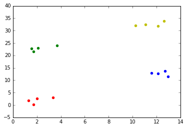
Suppose we have the following multiclass training set data
import copy

def generateMulticlassClassificationData():

    x = [np.zeros(shape=4), np.zeros(shape=4), np.zeros(shape=4), np.zeros(shape=4)]
    y = copy.deepcopy(x)

    for i in range(0, len(x)):
        x_offset = (i % 2) * 10
        y_offset = i * 10
        x1 = x[i]
        y1 = y[i]
        x1[0] = 1 + x_offset + np.random.uniform(0, 2) - 1
        y1[0] = 2 + y_offset + np.random.uniform(0, 2) - 1
        x1[1] = 2 + x_offset + np.random.uniform(0, 2) - 1
        y1[1] = 3 + y_offset + np.random.uniform(0, 2) - 1
        x1[2] = 2 + x_offset + np.random.uniform(0, 2) - 1
        y1[2] = 1 + y_offset + np.random.uniform(0, 2) - 1
        x1[3] = 3 + x_offset + np.random.uniform(0, 2) - 1
        y1[3] = 3 + y_offset + np.random.uniform(0, 2) - 1

    return x, y

def plotScatterData(x, y):
    color = {
        0: 'r',
        1: 'b',
        2: 'g',
        3: 'y'
    }
    for i in range(0, len(x)):
            plt.scatter(x[i], y[i], color=color[i])
    plt.show()

x, y = generateMulticlassClassificationData()
plotScatterData(x, y)
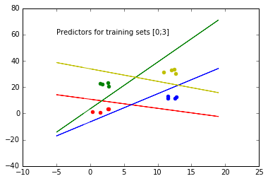
The following code implements a one vs. all logistic regression approach
def gradientDescentMC(x, y, setIndex, alphaFactor, numIterations):
    theta = np.ones(3)
    x_transposed = np.array([item for sublist in x for item in sublist]).transpose()
    y_transposed = np.array([item for sublist in y for item in sublist]).transpose()

    yl = [int(set == setIndex) for set, sublist in enumerate(y) for _ in sublist]
    n_samples = sum([len(set) for set in x])

    np.seterr(all='raise')  # Watch out for over/underflows

    for i in range(0, numIterations):

        sigmoid = lambda x: 1.0 / (1.0 + np.exp(-x))

        hypothesis = np.zeros(n_samples)
        offset = 0
        for set in range(0, len(x)): # We're keeping this verbose for readability's sake
            for sample in range(0, len(x[set])):
                hypothesis[offset + sample] = sigmoid(theta[0] + theta[1] * x[set][sample] + theta[2] * y[set][sample])
            offset += len(x[set])

        error_vector = hypothesis - yl

        gradient = np.zeros(3)
        gradient[0] = np.sum(error_vector) / n_samples
        gradient[1] = np.dot(x_transposed, error_vector) / n_samples
        gradient[2] = np.dot(y_transposed, error_vector) / n_samples

        theta = theta - alphaFactor * gradient

    return theta

'''
    Boilerplate plotting helpers
'''
def drawMCPredictors(theta_vector):
    color = {
        0: 'r',
        1: 'b',
        2: 'g',
        3: 'y'
    }
    plt.text(-5, 60, "Predictors for training sets [0;" + str(len(x) - 1) + "]")
    for i in range(0, len(x)):  # Graph all predictors
        y_regression = np.zeros(25)
        x_regression = np.zeros(25)
        for sample in range(-5, 20):
            x_regression[sample] = sample
            y_regression[sample] = -(theta_vector[i][0] + theta_vector[i][1] * sample) / theta_vector[i][2]
        plt.plot(x_regression, y_regression, color=color[i])

def getMCThetaVector(x, y):
    theta_vector = []
    for i in range(0, len(x)):
        theta_vector.append(gradientDescentMC(x, y, i, 0.01, 30000))
    return theta_vector

def plotScatterData(x, y):
    color = {
        0: 'r',
        1: 'b',
        2: 'g',
        3: 'y'
    }
    for i in range(0, len(x)):
        plt.scatter(x[i], y[i], color=color[i])
    plt.show()

x, y = generateMulticlassClassificationData()
theta_vector = getMCThetaVector(x, y)
drawMCPredictors(theta_vector)
plotScatterData(x, y)
New samples will be classified according to
\[\max_{i} h_\theta^{(i)}(x)\]where \(i\) is the class that maximizes \(h_\theta(x)\).
Considerations
Other advanced algorithms are available for logistic regression tasks, for instance conjugate gradient or BFGS to solve unconstrained nonlinear optimization problems. Upside is speed and no need to choose an \(\alpha\) parameter, downside is usually the added complexity to implement them.