Linear regression
(This post is also available as a Jupyter notebook file here)
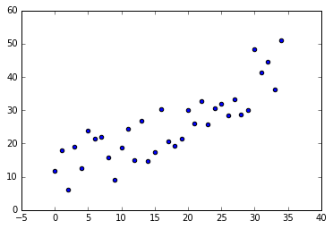
Linear regression is a mathematical approach to modeling the unknown parameters of linear predictor functions from data estimates. Let’s suppose we have a discrete uniformly distributed set of data (we’ll apply an ongoing bias and a spreading factor to better model an event sampling)
%matplotlib inline
import matplotlib.pyplot as plt
import numpy as np

# Generate N samples in range [0;1[ with a uniform distribution
def generateRandomData(numberOfSamples):
    x = np.zeros(shape=numberOfSamples)
    y = np.zeros(shape=numberOfSamples)

    for i in range(0, numberOfSamples):
        x[i] = i
        # Generates values along a line with a fixed degree of variance
        y[i] = i + np.random.uniform(0, 1) * 20

    return x, y

def plotScatterData(x, y):
    plt.scatter(x, y)
    plt.show()

x, y = generateRandomData(35)
plotScatterData(x, y)
In the case for a linear regression (linear polynomial) we’re interested in determining the parameters \(\theta_1\) and \(\theta_2\) for the hypothesis \(h_\theta(x)\) defined as
\[h_\theta(x) = \theta_0 + \theta_1x\]If we define a generic \(h_\theta(x)\) by assigning, for instance, \(\theta_1 = 1\) and \(\theta_2 = 1\), we will have an error that can be estimated by using the sum of the squared error method
\[J(\theta_1, \theta_2)=\sum^{m}_{i=1}{(h_\theta(x^{(i)}) - y^{(i)})^2}\]and therefore the optimization problem we need to solve is finding \(min \ J(\theta_1, \theta_2)\)
Gradient Descent
A straightforward approach to solving the optimization problem explained in the previous paragraph is the gradient descent method. The idea is to compute \(\nabla J(\theta_1, \theta_2)\) and use it as a negative gradient to find the decreasing direction of the multi-variable function J.
Therefore (we’re adding a \(\frac{1}{2m}\) factor to simplify computation)
\[\begin{align} & \frac{\partial}{\partial \theta_1}J(\theta_1, \theta_2) = \frac{1}{m} \sum^{m}_{i=1}{(h_\theta(x^{(i)}) - y^{(i)})} \\ & \frac{\partial}{\partial \theta_2}J(\theta_1, \theta_2) = \frac{1}{m} \sum^{m}_{i=1}{(h_\theta(x^{(i)}) - y^{(i)}) x^{(i)}} \end{align}\]If we choose a suitable \(\alpha\) factor (the learning rate) for the descent in the \(-\nabla\) direction (a compromise between convergence speed and actually converging to a function minimum), the algorithm becomes
while(!converged) {
  theta1 = theta1 - alpha * nabla[0];
  theta2 = theta2 - alpha * nabla[1];
  // Verify convergence
}
def gradientDescent(x, y, alphaFactor, numIterations):
theta = np.ones(2)
x_transposed = x.transpose()
n_samples, = np.shape(x)
np.seterr(all='raise') # Watch out for overflows
for i in range(0, numIterations):
hypothesis = np.zeros(n_samples)
for sample in range(0, n_samples):
hypothesis[sample] = theta[0] + theta[1] * x[sample]
error_vector = hypothesis - y
gradient = np.zeros(2)
gradient[0] = np.sum(error_vector) / n_samples
gradient[1] = np.dot(x_transposed, error_vector) / n_samples
theta = theta - alphaFactor * gradient
return theta
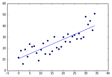
def plotLinearPredictor(x, y, theta_coefficients):
plt.scatter(x, y)
y_regression = np.zeros(len(x))
for sample in range(0, len(x)):
y_regression[sample] = theta_coefficients[0] + theta_coefficients[1] * x[sample]
plt.plot(x, y_regression)
plt.show()
theta_coefficients = gradientDescent(x, y, 0.001, 100000)
plotLinearPredictor(x, y, theta_coefficients)
Multivariate gradient descent
The generalized version for multiple features is
\[\forall \ j \quad \theta_j = \theta_j - \alpha \frac{\partial}{\partial \theta_j}J(\theta_1, \theta_2, \cdots, \theta_n) = \frac{1}{m} \sum^{m}_{i=1}{(h_\theta(x^{(i)} - y^{(i)})^2} x^{(i)}_j\]where \(x^{(i)}_j\) is the \(j\)-th feature \(i\)-th sample.
Normal equation method
An analytical solution exists and as it is the common case in calculus it involves
\[\theta \in \mathbb R^{n+1} \quad \forall \ j \quad \frac{\partial}{\partial \theta_j}J(\theta) = 0\]although this is straightforward, there’s a simpler method to calculate the system solution vector. Let us define a design matrix and a \(y\) vector for the training data
\[X = \begin{bmatrix} X^{(1)}_0 & X^{(1)}_1 & \cdots & X^{(1)}_n \\ X^{(2)}_0 & X^{(2)}_1 & \cdots & X^{(2)}_n \\ \vdots & \vdots & \ddots & \vdots \\ X^{(m)}_0 & X^{(m)}_1 & \cdots & X^{(m)}_n \\ \end{bmatrix} \qquad y = \begin{bmatrix} y^{(1)} \\ y^{(2)} \\ \vdots \\ y^{(m)} \\ \end{bmatrix}\]It turns out that
\[\theta = (X^TX)^{-1} X^Ty\]def normEquation(x, y):
ll = []
for sample in x:
ll += [[1] + [sample]]
X = np.matrix(ll)
ll = [[sample] for sample in y]
y = np.matrix(ll)
x_trans = X.T
A = (x_trans * X).I
theta = A * x_trans * y
return theta
theta_coefficients = normEquation(x, y)
plotLinearPredictor(x, y, theta_coefficients)

Considerations
The normal equation method doesn’t require an iterative approach and doesn’t need features adjustments like feature scaling, mean normalization or learning rate adjustment either. Downside is that the normal equation method doesn’t scale well with a huge number of features (big matrix inversion ~ doesn’t scale up well).