Separable kernel constituent vectors
GPU image processing operations can often be renderered substantially faster when using a separable kernel. Separable kernels are the result of tensor product between constituent vectors and have rank 1. The constituent vectors can be found by singular value decomposition, anyway in this article we’ll present an alternative approach.
The key observation is that all their rows and columns are multiple of the constituent vectors i.e. all of their elements are of the form \( m_{i,j} = a_i k \) where \( k \) is a multiplicative constant for the row or the column being considered.
\[v_1 \left[ \begin{array}{ccc} 3\\4\\1 \end{array} \right] \bigotimes v_2 \left[ \begin{array}{ccc} 2&8&3 \end{array} \right] = m \left[ \begin{array}{ccc} 6&24&9\\ 8&32&12\\ 2&8&3 \end{array} \right]\]The first step in reconstructing the constituent vectors is therefore to find
the greatest common divisor
in a row (the same reasoning will apply for columns). Dividing all elements by
the gcd will reduce them in the form \( a_i \).
After performing the same computations for columns an additional observation has to be made: we’re searching constituent vectors for the original known matrix, that means we’re interested in having \( x_i \cdot y_j = m_{i,j}\). In a case like the following the algorithm we’re using won’t work
\[v_1 \left[ \begin{array}{ccc} 6\\12 \end{array} \right] \bigotimes v_2 \left[ \begin{array}{ccc} 6&27 \end{array} \right] = m \left[ \begin{array}{ccc} 36&72\\ 162&324 \end{array} \right]\]since it will yield
\[v_1 \left[ \begin{array}{ccc} 1\\2 \end{array} \right] v_2 \left[ \begin{array}{ccc} 2&9 \end{array} \right]\]a scale factor of \( \frac{m_{i,j}}{x_i \cdot y_j} \) is needed on one of the constituent candidates.
Finally the python algorithm to compute the constituent vectors follows
import numpy as np
from mpl_toolkits.mplot3d import axes3d
import matplotlib.pyplot as plt
from matplotlib import cm
'''
This code demonstrates that a Gaussian kernel M of rank 1 is also
separable and can be obtained as the tensor product of two vectors
X and Y
'''
def gcd(x, y):
if x == 0:
return y
else:
return gcd(y % x, x)
# Separate a 2D kernel m into x and y vectors
# Returns [bool valid, x, y] with valid set to True if it was possible
# to find two valid constituent x and y vectors
def separate(m):
x = np.squeeze(np.asarray(m[0, :]))
y = np.squeeze(np.asarray(m[:, 0]))
nx = x.size
ny = y.size
gx = x[0]
for i in range(1, nx):
gx = gcd(gx, x[i])
gy = y[0]
for i in range(2, ny):
gy = gcd(gy, y[i])
x = x / gx
y = y / gy
scale = m[0, 0] / (x[0] * y[0])
x = x * scale
valid = np.allclose(np.outer(y, x), m)
return valid, x, y
# Usage example
# |3| |6 24 9|
# |4| * |2 8 3| == |8 32 12|
# |1| |2 8 3|
mat = np.outer([[3], [4], [1]], [[2, 8, 3]])
separate(mat)
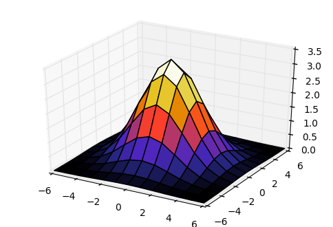
# Generate a symmetric separable Gaussian kernel of radius size (w==h==2*size+1)
def generate_gaussian_kernel(size, sigma = 3, central_value = 3.5, center=None):
# Generate a size x size grid
a = np.linspace(-size, size, 2 * size + 1)
b = a
x, y = np.meshgrid(a, b)
return x, y, np.exp(-(x / sigma)**2 - (y / sigma)**2) * central_value
xgrid, ygrid, mat = generate_gaussian_kernel(6)
fig = plt.figure()
ax = fig.add_subplot(111, projection='3d')
ax.plot_surface(xgrid, ygrid, mat, rstride=1, cstride=1, cmap='CMRmap')
plt.show()
if np.linalg.matrix_rank(mat) == 1:
valid, x, y = separate(mat)
if valid:
print "Constituent vectors found: \nv1:", x, '\nv2:', y
else:
print "Constituent vectors not found"
else:
print "Not a rank 1 matrix"
Constituent vectors found:
v1: [  2.16840434e-19   7.36113251e-19   2.00096327e-18   4.35535655e-18
 7.59099013e-18   1.05940801e-17   1.18390866e-17   1.05940801e-17
 7.59099013e-18   4.35535655e-18   2.00096327e-18   7.36113251e-19
 2.16840434e-19]
v2: [  5.41466909e+15   1.83813027e+16   4.99655611e+16   1.08756536e+17
 1.89552745e+17   2.64542166e+17   2.95630915e+17   2.64542166e+17
 1.89552745e+17   1.08756536e+17   4.99655611e+16   1.83813027e+16
 5.41466909e+15]