Matrix chain multiplication - MCOP
Matrix multiplication is a fundamental problem in linear algebra.
Given a \( A \times B \) matrix and a second \( B \times C \) matrix, the result of their multiplication is a \( A \times C \) matrix with its elements calculated by the following naive code
#include <iostream>
#include <vector>
#include <iterator>

int main() {

  std::vector<std::vector<int>> matrix1 = { // 2 x 4
    { 1, 2, 3, 4 },
    { 5, 6, 7, 8 }
  };

  std::vector<std::vector<int>> matrix2 = { // 4 x 3
    { 1, 2, 3 },
    { 4, 5, 6 },
    { 7, 8, 9 },
    { 10, 11, 12 }
  };

  const size_t A = matrix1.size();
  const size_t B = matrix2.size(); // Matrices must have this dimension in common
  const size_t C = matrix2[0].size();

  // matrix1 is A x B
  // matrix2 is B x C

  // Matrix multiplication. The resulting matrix is
  // (A x B) x (B x C) = A x C
  std::vector<std::vector<int>> result(A, std::vector<int>(C, 0));

  for (size_t a = 0; a < A; ++a) {
    for (size_t c = 0; c < C; ++c) {
      for (size_t b = 0; b < B; ++b) {
        result[a][c] += matrix1[a][b] * matrix2[b][c];
      }
    }
  }

  // Print out resulting matrix
  for (auto& v : result) {
    std::copy(v.begin(), v.end(), std::ostream_iterator<int>(std::cout, " "));
    std::cout << std::endl;
  }

  return 0;
}
The loop performs a grand total of \( A \times B \times C \) multiplications. Keep this amount in mind for the rest of the article.
The cost of matrix multiplication
When multiplying a (possibly large) chain of matrices together, if they’re not all of the same dimension, there is a way to increase computation performances.
Matrix multiplication is not commutative but it is associative, that means
\[(X \times Y) \times Z = X \times (Y \times Z)\]i.e. we can decide which multiplication should be executed first.
Turns out this actually pays off if the dimensions are sufficiently irregular and we multiply chains of matrices often enough. Assume that we have three matrices \( X,Y,Z \) with dimensions \( 2 \times 4 \), \( 4 \times 3 \) and \( 3 \times 7 \) and recall from above the number of multiplications necessary to multiply two matrices.
Depending on how we parenthesize the multiplication expression we get a different number of operations to be performed
\[(X \times Y) \times Z \\ ([2 \times 4] \times [4 \times 3]) \times [3 \times 7] \\ (2 \times 4 \times 3 \ multiplications) for \ a \ 2 \times 3 \ matrix \\ + 2 \times 3 \times 7 \ multiplications \ for \ the \ final \ 2 \times 7 \ matrix = 24 + 42 = 66\]against
\[X \times (Y \times Z) \\ [2 \times 4] \times ([4 \times 3] \times [3 \times 7]) \\ (4 \times 3 \times 7 \ multiplications) for \ a \ 4 \times 7 \ matrix \\ + 2 \times 4 \times 7 \ multiplications \ for \ the \ final \ 2 \times 7 \ matrix = 84 + 56 = 140\]Thus, in the example above, the best ‘parenthesization’ is \( (X \times Y) \times Z \).
Naive algorithm to find the minimum number of multiplications for a matrix chain
A simple (and somewhat inefficient) algorithm to find the number of minimum multiplications necessary for a matrix chain is the following
#include <iostream>
#include <vector>

int minimumNumberOfMultiplications(std::vector<int>& dimVec, int start, int end) {

  if (start >= end)
    return 0; // Cost is 0 (neuter element for addition) when this is an invalid range

  int minFound = std::numeric_limits<int>::max(); // The minimum cost found

  // Place a parenthesis break from 0 to k. E.g.
  // 2 4 3 7 with k = 1 means "Break from 0 to k including the element at k"
  // -> (2 4) 3 7
  // -> (2x4) 4x3 3x7
  for (int k = start; k < end; ++k) {
    // Every sub-parenthesized expression must yield a matrix of dimensions
    // dimVec[start] x dimVec[k].
    // We take advantage of this fact to "merge" the results of the recursions:
    // ( 2x4 4x3 ) (3x7)
    // ^^^^^^^^^^^
    // This yields a 2x3 matrix. The other parenthesis yields a 3x7 matrix.
    // The above can be written as
    //  minimumNumberOfMultiplications( (2x4 4x3) ) +
    //  minimumNumberOfMultiplications( (3x7 ) +
    //  merge price of a 2x3 x 3x7 matrix join -> 2*3*7 operations
    int newMin = minimumNumberOfMultiplications(dimVec, start, k) +
                 minimumNumberOfMultiplications(dimVec, k + 1, end) +
                 dimVec[start - 1] * dimVec[k] * dimVec[end];

    if (newMin < minFound)
      minFound = newMin;
  }

  return minFound;
}

int main() {
  std::vector<int> matrixDimensions = { 2, 4, 3, 7 }; // Three matrices: 2x4, 4x3, 3x7

  std::cout << "Minimum number of multiplications for the input sized matrices is "
            << minimumNumberOfMultiplications(matrixDimensions, 1,
                static_cast<int>(matrixDimensions.size() - 1)); // 66

  return 0;
}
Caveats:
- Be careful with the termination conditions. In particular the trivial no-parenthesis-necessary case (or everything-parenthesized) \( (A) \times (B) \times (C) \) is already handled thanks to the recursion
- Recall the amount of multiplications necessary to understand the main loop statement
The loop performs a grand total of \( A \times B \times C \) multiplications. Keep this amount in mind for the rest of the article.
The solution proposed works but it is quite slow and has exponential time bounded by \( O(2^n) \).
By observing the case above with dimensions \( 2 \times 4 \), \( 4 \times 3 \) and \( 3 \times 7 \), the partial recursion looks like the following
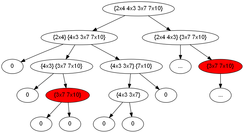
Notice the red nodes as being overlapping subproblems. This means the problem is a good candidate to be solved with a dynamic programming solution.
Dynamic programming
First it has to be noted that storing the intermediate results in a dynamic programming fashion will require two dimensions: we must be able to store the minimum found for each \( f(i,j) \) call where \( i \) is the start of a subexpression and \( j \) the end of it. Thus we’ll require a 2D matrix for memoization.
Then in order to have all the partial results available when we need it, we must first construct the subproblems that directly rely on the base cases (i.e. subexpression of just one matrix): these are the subexpressions of length 2. The subexpressions of length 3 will rely on the subexpressions of length 2 and so forth.
#include <iostream>
#include <vector>
#include <limits>
int minimumNumberOfMultiplications(std::vector<int>& dimVec) {
// A memoization matrix of NxN
const size_t N = dimVec.size();
std::vector<std::vector<int>> matrix(N, std::vector<int>(N, 0));
// Base cases: 1-length subexpressions
// Code is unnecessary (included in the zero-initialization above)
// for (int i = 0; i < N; ++i) {
// matrix[i][i] = 0;
// }
// For every subexpression length
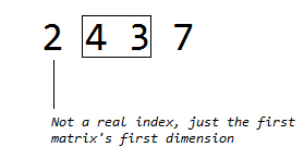
for (int l = 2; l <= N - 1 /* First element is not a real element */; ++l) {
for (int i = 1; i <= N - l; ++i) { // For every beginning i
int j = i + l - 1; // And get the subexpression ending too
int minFound = std::numeric_limits<int>::max();
for (int k = i; k < j; ++k) {
int newMin = matrix[i][k] + matrix[k + 1][j] +
dimVec[i - 1] * dimVec[k] * dimVec[j]; // See quote
if (newMin < minFound)
minFound = newMin;
}
matrix[i][j] = minFound; // Store the minimum obtained for this interval
}
}
return matrix[1][N - 1];
}
int main() {
std::vector<int> matrixDimensions = { 2, 4, 3, 7 }; // Three matrices: 2x4, 4x3, 3x7
std::cout << "Minimum number of multiplications for the input sized matrices is "
<< minimumNumberOfMultiplications(matrixDimensions); // 66
return 0;
}The code above uses dynamic programming to slide a window of two elements (one element has a trivial minimum solution of 0 multiplications necessary) from the first valid element (i.e. the 1-index element since the first is not a valid element but rather the first matrix’s first dimension) forward while the window fits.
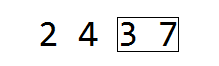
At each iteration of the i loop the window slides forward
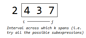
The k loop works in the same way as the naive method and just searches recursively for a minimum in the right/left partitions in the \( (i;j) \) interval.
In the example above the last window to be calculated is the one comprising all the elements
The final minimum value will be available by querying the memoization table for the entire interval
\[min f(i,j) = matrix[i][j]\] \[\Rightarrow minf(1,N-1) = matrix[i][N-1]\]The dynamic programming solution is \( O(n^3) \) but still proves to be much faster than the naive approach.